A structural detail is subjected to a stress range of 100 MPa at N = 10⁶ cycles. Is this acceptable?
The answer most engineers give — if they have some familiarity with fatigue design — is to check whether 100 MPa is below the allowable stress for the applicable FAT class. If this is a fillet weld toe on a plate edge, the allowable stress range at 10⁶ cycles is approximately 107 MPa for FAT 80. The detail passes.
But the question is poorly framed — and the fact that it is poorly framed is itself the signal. In offshore fatigue design, you almost never assess a detail against a single stress range at a single cycle count. You assess it against a loading spectrum — a distribution of stress ranges, each occurring a different number of times, over the design life. The question is not “does this detail survive 10⁶ cycles at 100 MPa?” The question is “does this detail survive the cumulative damage from 10⁶ cycles at 80 MPa, plus 5×10⁵ cycles at 120 MPa, plus 2×10⁵ cycles at 150 MPa, plus all the other stress events in the spectrum, without the cumulative damage exceeding 1.0?”
Getting to that question — and knowing how to answer it — requires understanding how FAT classes are defined, how S-N curves are constructed, what the slope change at high cycle counts means, and how Miner’s rule works in practice. This post covers the things that are most commonly misapplied.
What FAT Actually Means
FAT is not a material property. It is not a steel grade. It is a detail classification — a number that indexes an S-N curve to a specific welded joint geometry.
The FAT number is defined as the allowable stress range in megapascals at N = 2×10⁶ cycles. This is important: the reference cycle count is 2×10⁶, not 10⁶. Confusion between these two cycle counts is one of the most common errors in fatigue design. The fatigue limit sometimes cited at 10⁶ cycles in undergraduate texts is a different concept — it refers to the approximate knee of the S-N curve for unwelded parent material. The FAT class is defined at 2×10⁶ because that is the reference cycle count used in DNV-RP-C203, and that is the standard that governs offshore fatigue design in the North Sea and most international offshore jurisdictions.
FAT 80 means: at N = 2×10⁶ cycles, the allowable stress range is 80 MPa. FAT 100 means: at the same cycle count, the allowable stress range is 100 MPa. The higher the FAT number, the more fatigue-resistant the detail category.
The FAT class hierarchy in DNV-RP-C203 runs from FAT 71 (most severe — fillet weld toe on structural tee, unsupported) to FAT 125 (least severe — unwelded parent material). The progression is not arbitrary. It reflects the severity of the stress concentration at the crack-prone location in each detail type.
Why FAT Class Is Determined by Geometry, Not by Steel Grade
A question that arises regularly: does higher-strength steel give a better FAT class?
No. S355 and S690 steel, welded into the same joint geometry, receive the same FAT class. FAT class is a function of stress concentration geometry — the local stiffness and geometry of the welded connection — not the parent material yield strength. A FAT 80 joint in S355 and a FAT 80 joint in S690 have the same fatigue performance in terms of allowable stress range at a given cycle count. The higher-strength steel does not compensate for a poor joint geometry. The geometry is what matters.
This is why offshore fabrication specifications require specific weld toe profiles, minimum leg sizes, and in some cases weld toe grinding and MPI inspection — not because the weld needs to be stronger in a yield sense, but because the weld toe geometry determines the FAT class, which determines the allowable stress range, which determines the fatigue life.
The S-N Curve: How the FAT Class Defines the Curve
The FAT class defines the intercept of the S-N curve on the stress axis. The slope is m = 3 for N < approximately 5×10⁶ cycles (the high-cycle regime). The governing equation is:
N = C / Δσ^m
where C is a constant derived from the FAT class. The relationship between FAT class and C is:
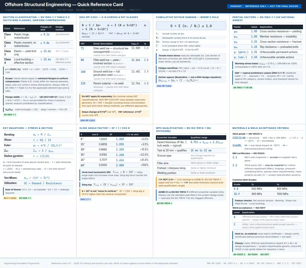
| FAT Class | log₁₀ C | C |
|---|---|---|
| FAT 71 | 12.000 | 10¹²·⁰⁰⁰ |
| FAT 80 | 12.164 | 10¹²·¹⁶⁴ |
| FAT 100 | 12.481 | 10¹²·⁴⁸¹ |
| FAT 125 | 12.764 | 10¹²·⁷⁶⁴ |
Using the correct C value matters. If you use the wrong C — for example, applying C = 10¹²·⁰⁰⁰ (FAT 71’s value) to a FAT 100 detail — you will under-predict the allowable stress range for FAT 80, FAT 100, and FAT 125 details and produce an unconservative fatigue assessment.
For a FAT 100 detail at N = 10⁶ cycles: Δσ_all = (C/10⁶)^(1/3) = (10¹²·⁴⁸¹/10⁶)^(1/3) = 10²·¹⁶⁰ ≈ 144 MPa. If you had mistakenly used C = 10¹²·⁰⁰⁰, you would get Δσ_all ≈ 126 MPa — a 13% error in the allowable stress range, in the conservative direction for this case. At higher cycle counts, the error grows.
The Slope Change at 5×10⁶ Cycles
Below approximately 5×10⁶ cycles, the S-N curve for most offshore detail categories follows m = 3. Above 5×10⁶ cycles, the slope steepens to approximately m = 5. This is not a minor technical footnote — it is the difference between a fatigue assessment that passes and one that significantly underestimates fatigue damage.
The reason for the slope change is metallurgical: at very high cycle counts, the fatigue mechanism shifts from the formation and propagation of a dominant crack to the simultaneous initiation of multiple micro-cracks. The effective stress intensity at the crack tip reduces, and the growth rate per cycle drops. The m = 5 slope above 5×10⁶ reflects this different mechanism.
In cumulative damage calculations using Miner’s rule, this slope change means that stress ranges in the very high-cycle regime contribute less damage per cycle than the m = 3 extrapolation would predict. But it also means that if your loading spectrum includes a large number of cycles in the 10⁶ to 10⁷ range — as many offshore structures do — the fatigue assessment must use the correct slope for each portion of the spectrum.
Request our complimentary Structural Engineering Reference Card
Cumulative Damage: Miner’s Rule in Practice
Miner’s rule is the standard method for combining fatigue damage from multiple stress ranges:
D = Σ (nᵢ / Nᵢ) ≤ 1.0
where nᵢ is the number of cycles applied at stress range Δσᵢ, and Nᵢ is the allowable cycles at that stress range from the S-N curve. The damage sum D must not exceed 1.0 for the design life.
In practice, applying Miner’s rule requires a stress spectrum — a histogram of stress ranges and their frequencies of occurrence. For offshore structures, this is usually derived from a wave scatter diagram combined with a structural analysis that gives the stress range at the detail per wave height and period. The result is a damage sum, not a binary pass/fail at a single stress level.
The important caveat: Miner’s rule is a linear damage accumulation hypothesis. It assumes damage is independent of load sequence and that the damage contribution from each stress range is additive. In reality, load sequence effects exist — compressive overloads can retard subsequent crack growth, tensile overloads can accelerate it. DNV-RP-C203 acknowledges this and requires consideration of load sequence effects for details where compressive overloads are expected, which is routine in offshore fatigue loading from storm conditions.
Common Errors and How to Avoid Them
Error 1: Using the FAT number at the wrong cycle count. FAT 80 does not mean 80 MPa at 10⁶ cycles. It means 80 MPa at 2×10⁶ cycles. Always check what the reference cycle count is in the code you are using.
Error 2: Applying a stress concentration factor Kt in addition to the FAT class. DNV-RP-C203 already incorporates the stress concentration effect into the FAT class definition. Do not apply Kt to the nominal stress before comparing against the FAT class S-N curve — that is double-counting the stress concentration.
Error 3: Ignoring the mean stress correction for tensile mean stresses. The basic S-N curve is for zero-mean (alternating) stress. For tensile mean stresses, the allowable stress range is reduced. DNV-RP-C203 provides mean stress correction factors. In the high-cycle regime, this correction can be significant.
Error 4: Using the same slope for all cycle ranges. The m = 3 slope only applies below 5×10⁶ cycles for most detail categories. Above that, use m = 5.
Where This Fits in Practice
FAT class selection and S-N curve application is Week 2 of our Engineering Foundation Programme — taught after the structural fundamentals week, before the welding and materials weeks, because fatigue design affects connection detailing, weld quality requirements, and materials selection throughout the rest of the programme.
The FAT class system is not a standalone topic. It connects directly to weld quality requirements (how smooth the weld toe needs to be to achieve FAT 100 versus FAT 80), to inspection strategy (which details warrant ultrasonic examination of the weld toe after fabrication), and to in-service inspection requirements (which details should be included in an underwater inspection programme on a fixed platform).
Understanding FAT class selection is understanding why offshore fabrication specifications are written the way they are.
The FAT class system and its correct application is Week 2 of our Engineering Foundation Programme, taught with reference to DNV-RP-C203 and applied to worked examples drawn from real offshore connection details. Week 2 also covers brittle fracture, the weld toe fatigue mechanism, and cumulative damage calculations using Miner’s rule.
[See this link for more information→] Offshore and Mechanical Engineering Training Programme
Find out more, fill in your contact details below and we will come back to you as soon as possible.